Basic of Ms Excel

Microsoft Excel is a spreadsheet program that is used to store, sort and efficiently crunch numbers. Accountants use Excel to keep track of transactions for their company.

Create a new workbook

Excel documents are called workbooks.Each workbook has sheets, typically called spreadsheets. You can add as many sheets as you want to a workbook, or you can create new workbooks to keep your data separate.

Click File > New.

Under New, click the Blank workbook.

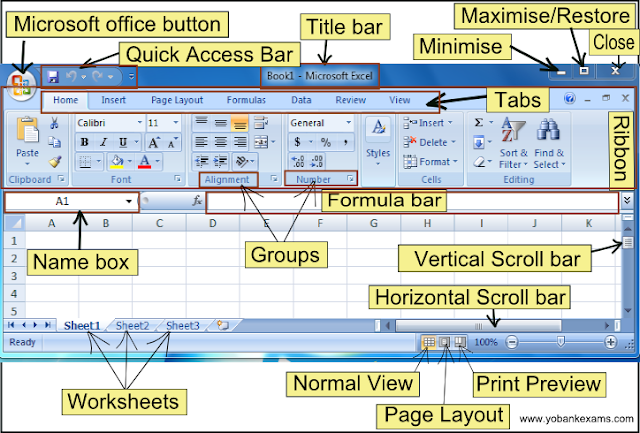
• Microsoft office button:This is a round button that you can see on the uppermost left corner of the workbook.You can use this to open a new workbook or save.We will be exploring the options under this head in detail in the next lesson.

• Quick Acess Toolbar:There is a small bar right next to the Microsoft Office button.You can customise and add frequently used commands to the quick access tool bar so that you access any command at a click.

• Title bar:Title bar appears at the top of any worksheet.
• By default the 1st sheet you open is named as Book1 which you can rename by saving it with a different name.

• Minimise:There is minus(-)like symbol to the topmost right corner of the worksheet which you can use to minimise the window

• Maximise/Restore down:Next to the minimise button is a box shaped button which you can use to maximise or restore the window.

• Close:Next to Maximise button is Cross(x)sign which you can use to close the window.

• Ribbon:The whole area to the bottom of the title bar is the Ribbon.

• Tabs:Ribbon is divided into different tabs based on the functions they perform.We have the Home tab,Insert tab,Pagelayout tab,Formulas tab,Data tab, Review tab, View tab.

• Groups;All similar type of commands are grouped together into a group.
• Ex:Alignment and Number are groups.

• Name box:To the left corner below the Ribbon is the name box which shows the active cell/cell reference.

• Formula bar:The white area next to fx is the formula bar which you can use to insert formulas.

• Vertical scroll bar:To right of the worksheet is the vertical scroll bar which you can use to scroll to see more data on the vertical side.  

• Horizontal scroll bar:To the bottom right of the worksheet is the horizontalscroll bar which you can use to scroll to see more data on the horizontal side.

• Normal View:Below the horizontal scroll bar there is an icon called normal view which you can use to view the worksheet in the normal mode.

• Page Layout:Below the horizontal scroll bar there is another icon in the middle called Page Layout which allows you to modify the page layout.

• Print Preview:Below the horizontal scroll bar next to Page layout is the Print Preview button which shows you how the worksheet looks when you print it.

Enter your data

Click an empty cell. For example, cell A1 on a new sheet.

Cells are referenced by their location in the row and column on the sheet, so cell A1 is in the first row of column A.

Type text or a number in the cell.

Press Enter or Tab to move to the next cell.

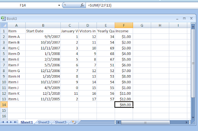
Use AutoSum to add your data

When you’ve entered numbers in your sheet, you might want to add them up. A fast way to do that is by using AutoSum.

Select the cell to the right or below the numbers you want to add.

Click Home > AutoSum, or press Alt+=.

AutoSum adds up the numbers and shows the result in the cell you selected.

Create a simple formula

Adding numbers is just one of the things you can do, but Excel can do other math too. Try some simple formulas to add, subtract, multiply or divide your numbers.

Pick a cell and type an equal sign (=). That tells Excel that this cell will contain a formula.

Type a combination of numbers and calculation operators, like the plus sign (+) for addition, the minus sign (-) for subtraction, the asterisk (*) for multiplication, or the forward slash (/) for division.

For example, enter =2+4, =4-2, =2*4, or =4/2.

Press Enter. That runs the calculation.

You can also press Ctrl+Enter if you want the cursor to stay on the active cell.

Apply a number format

To distinguish between different types of numbers, add a format, like currency, percentages, or dates.

Select the cells that have numbers you want to format.

Click Home > Arrow next to General.

Pick a number format.

Put your data in a table

A simple way to access a lot of Excel’s power is to put your data in a table. That lets you quickly filter or sort your data for starters.

Select your data by clicking the first cell and dragging to the last cell in your data.

To use the keyboard, hold down Shift while you press the arrow keys to select your data.

Click the Quick Analysis button  in the bottom-right corner of the selection.

Click Tables, move your cursor to the Table button so you can see how your data will look. If you like what you see, click the button.

Now you can play with your data: Filter to see only the data you want, or sort it to go from, say, largest to smallest. Click the arrow Filter drop-down arrow in the table header of a column.

To filter data, uncheck the Select All box to clear all check marks, and then check the boxes of the data you want to show in your table.

Show totals for your numbers

Quick Analysis tools let you total your numbers quickly. Whether it’s a sum, average, or count you want, Excel shows the calculation results right below or next to your numbers.

Select the cells that contain numbers you want to add or count.

Click the Quick Analysis button  Quick Analysis button in the bottom-right corner of the selection.

Click Totals, move your cursor across the buttons to see the calculation results for your data, and then click the button to apply the totals.

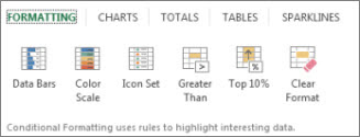
Add meaning to your data

Select the data you want to examine more closely.

Click the Quick Analysis button  that appears in the lower-right corner of your selection.

Explore the options on the Formatting and Sparklines tabs to see how they affect your data.

For example, pick a color scale in the Formatting gallery to differentiate high, medium, and low temperatures.

When you like what you see, click that option.

Show your data in a chart

The Quick Analysis tool recommends the right chart for your data and gives you a visual presentation in just a few clicks.

Select the cells that contain the data you want to show in a chart.

Click the Quick Analysis button  that appears in the lower-right corner of your selection.

Click Charts, move across the recommended charts to see which one looks best for your data, and then click the one that you want.

Save your work

Click the Save button on the Quick Access Toolbar, or press Ctrl+S.

Save button on the Quick Access Toolbar

If you’ve saved your work before, you’re done.

If this is the first time, go on to complete the next steps:

Under Save As, pick where to save your workbook, and then browse to a folder.

In the File name box, enter a name for your workbook.

Click Save to finish.

Print

Click File > Print, or press Ctrl+P.

Preview the pages by clicking the Next Page and Previous Page arrows.

The preview window displays the pages in black and white or in color, depending on your printer settings.

If you don’t like how your pages will be printed, you can change page margins or add page breaks.

Click Print.